
Accomplishments
- Improved Matching Efficiency
- Improved Matching Quality
- Minimum Spanning Tree With Maximum Confidence
- Feature Masking
Manually curating a few known-good images to be matched and processed is quick and relatively immune to false positives. However, applying that same manual process to 50+ images grinds workflows to a halt and quickly becomes strewn with incorrect matches. Without GPS or sequential metadata, chaotic image datasets suffer from the exponential performance scaling of any-to-any (n-choose-2) comparisons. This is especially painful for CPU-bound processes. Furthermore, this expanded dataset compounds the likelihood of introducing false positives that can slip through current feature-matching algorithms.
To effectively work with large datasets, we need to generate a minimum spanning tree where all images are connected, with high confidence regarding what each image matches to and exactly where those matches are located. Achieving this requires a multi-step approach: reducing CPU operations, iteratively filtering matches, and masking out corrupting environmental features like clouds and glass.
Improved Matching Efficiency
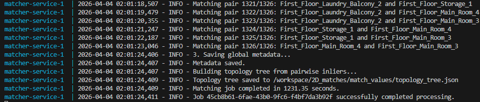
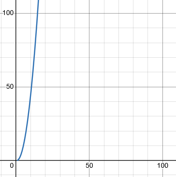
The fundamental purpose of the matching stage is to look at every photo and compare it against every other photo to find the best connections. Historically, our pipeline handled this in three steps: ALIKED (extracting specific pixels as features), LightGlue (comparing extracted pixels across every image in an any-to-any configuration), and Spherical RANSAC (converting images to spheres to validate matches without distortion). The problem? Matching any one photo to every other photo grows exponentially as the dataset scales. A small batch of just 52 photos requires over 1,300 unique comparisons.
Our primary bottleneck was Spherical RANSAC, a heavily CPU-bound operation. By switching from a standard Python library to a just-in-time (JIT) compiled version, we were able to execute the math directly on the hardware rather than pushing it through a Python abstraction layer. This single optimization cut the operation time by over 90%, bringing a 20+ minute process for 52 images down to just 2 or 3 minutes.
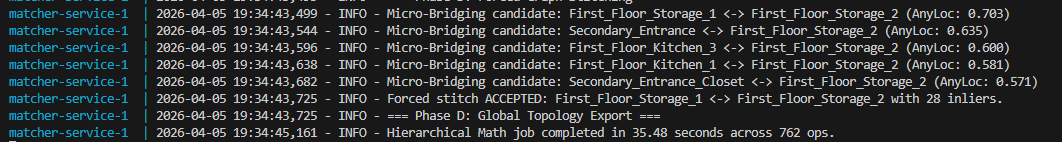
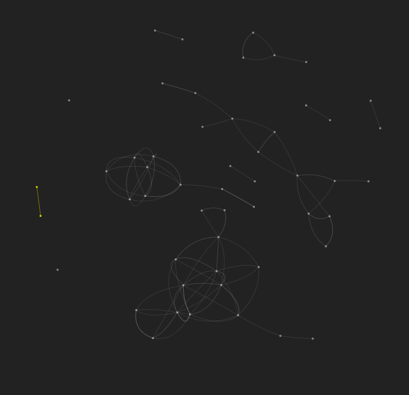
We also theorized using AnyLoc as a pre-check. AnyLoc is a “Global Descriptor”; instead of extracting individual features, it generalizes the image (e.g., turning a photo into a mathematical representation of “Inside, big bedroom, beige walls”). Because it runs entirely on the GPU, it is blazing fast, tearing through the 52 images in just 35 seconds. However, AnyLoc tends to group high-confidence matches by type rather than topology. It creates disconnected “islands” of similar rooms (like matching two separate bedrooms together) rather than finding the connective path (like a hallway leading to a bedroom). While AnyLoc is incredibly fast and worth considering for future iterations, its tendency to falsely combine distinct but similar rooms means it requires careful handling before full inclusion in the pipeline. Ultimately, by removing the abstraction bottleneck of our CPU process, we successfully reduced our overall matching speed by 95%.
Quality Improvement
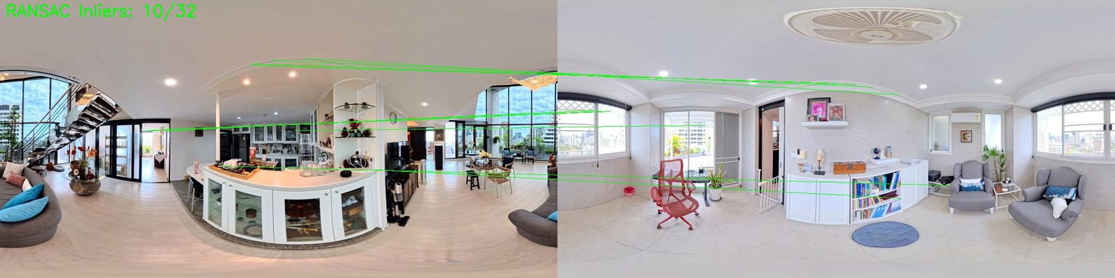
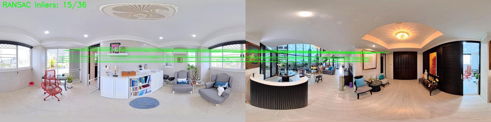
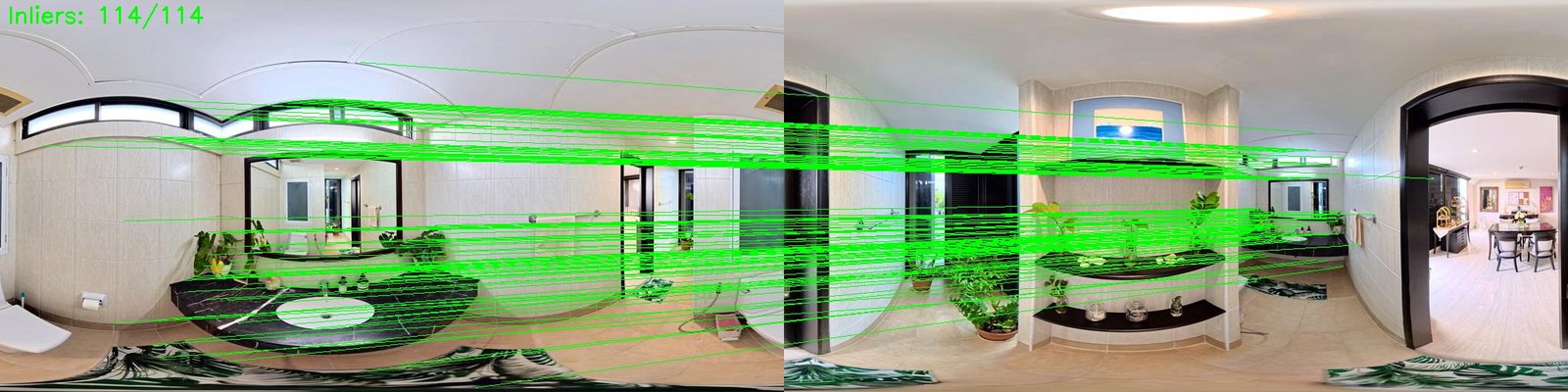
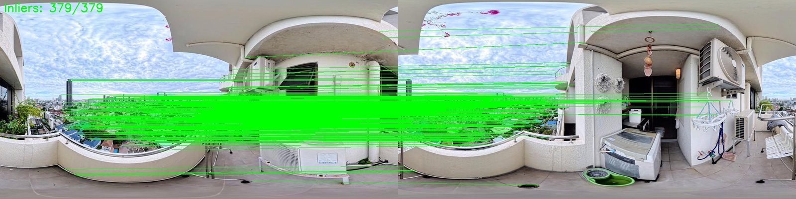
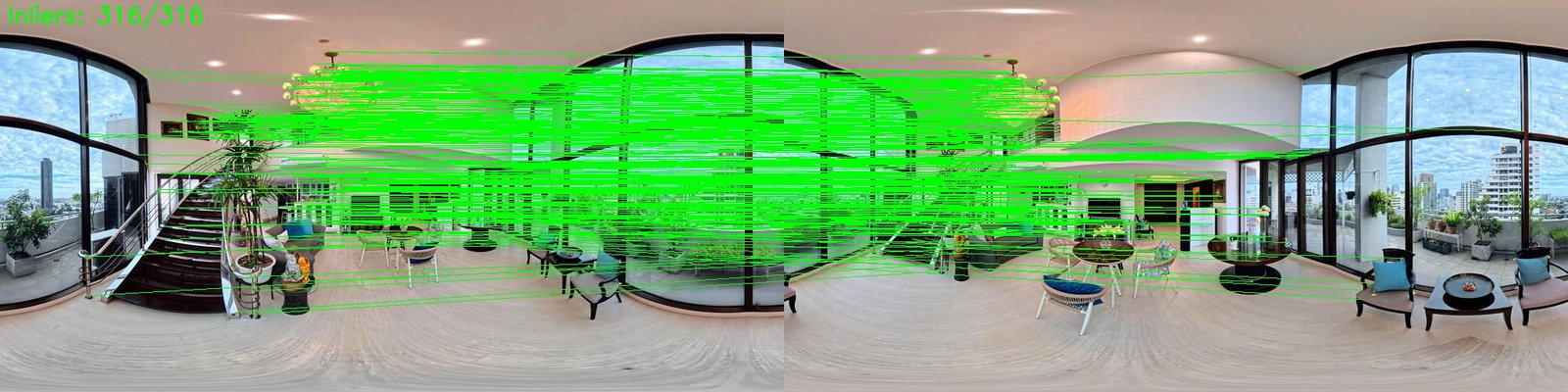
Speed is irrelevant if the feature matching yields incorrect results. The matches generated by LightGlue and Spherical RANSAC often include false positives. Two identical doors, two sides of a symmetrical feature, or even similar moldings and furniture in completely separate rooms can trick standard matchers into drawing a connection.
To solve this, we looked to RoMa V2 (Robust Matching), a dense feature matcher. What sets RoMa apart is its ability to rank every pixel in the image by confidence and match them at extreme angles. When we pass our challenging image pairs through RoMa V2, the false positive matches still appear, but they are flagged with remarkably low confidence scores and lack shared pixel density. This allows us to aggressively filter out the low-confidence noise while retaining dense, high-confidence pixel groups—even when looking through narrow doorways.
The trade-off for this accuracy is compute time. Dense matching requires dense math. RoMa V2 takes significantly longer than LightGlue, scaling exponentially and taking over 5 minutes for a 52-image dataset. Because of this, RoMa V2 is not a standalone silver bullet. It cannot process the entire dataset in a reasonable timeframe on its own, meaning we still rely on LightGlue as an early-stage filter to narrow down the workload before RoMa V2 confirms the final matches.
Minimum Spanning Tree & Maximum Confidence Path
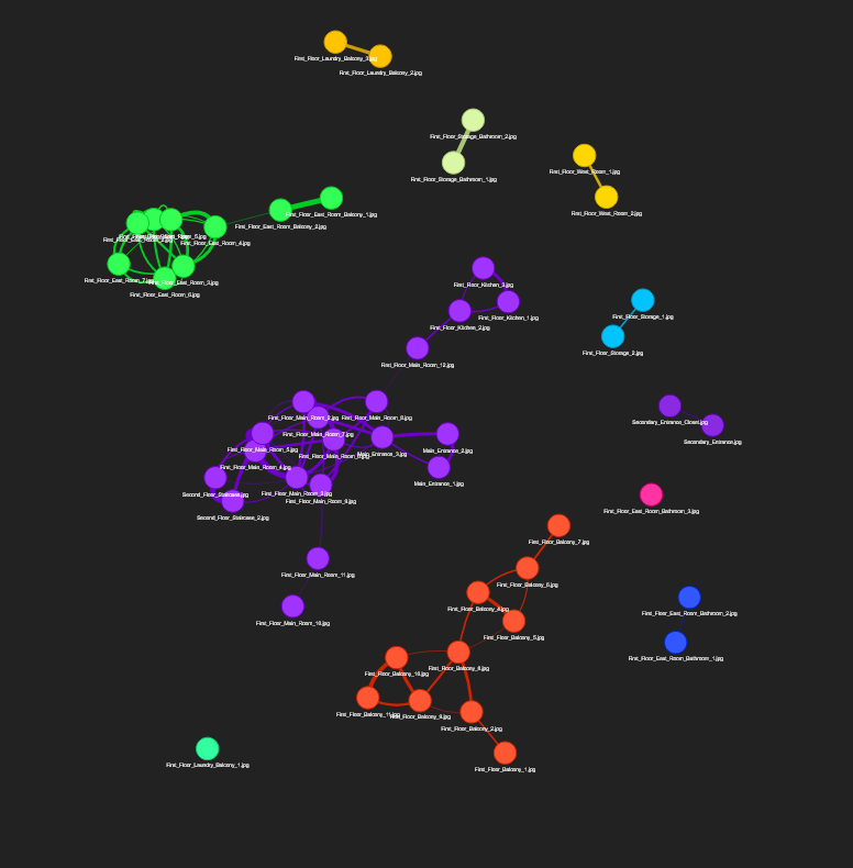
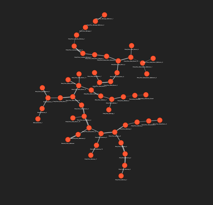
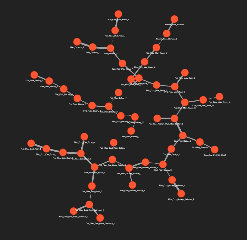
If we don’t confirm that every point cloud has valid matches and belongs to a unified tree of connections, we end up with incorrect geometry and floating, disconnected islands. LightGlue is reasonably fast, but its confidence scores for a correct match through a doorway might be identical to the score of a false positive between two disconnected rooms with similar moldings. RoMa V2 is the slowest, but it is the most accurate and provides the highest confidence for tricky bridges like doorways.
To get the minimum spanning tree with the highest confidence paths as quickly as possible, we re-architected the workflow to play to the strengths of both tools. First, we use LightGlue to perform the any-to-any matching and rank the pairs by confidence, narrowing down the field of likely candidates. We then intentionally skip the long Spherical RANSAC step, as RoMa V2 will handle match quality confirmation.
Next, we determine the top-ranked confidence values and begin building our topological tree. If any disconnected islands or orphaned nodes exist, we expand the tree to include slightly lower confidence values until a continuous path connects everything. Finally, RoMa V2 processes this curated list of rankings. It confirms the confidence values, outputs high-confidence dense matching points for each pair, and validates the bridges through doorways. This dual-model approach yields a unified minimum spanning tree connected entirely by maximum-confidence paths.
Feature Masking
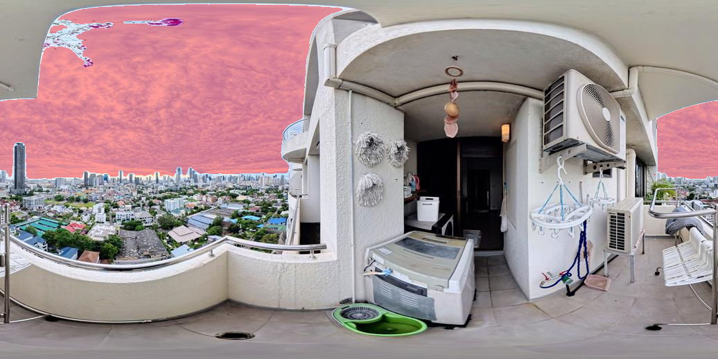
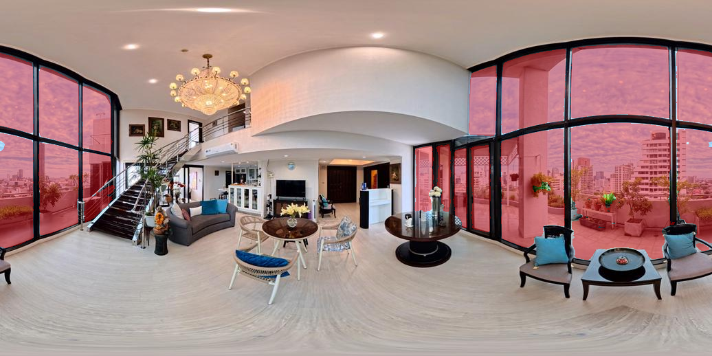
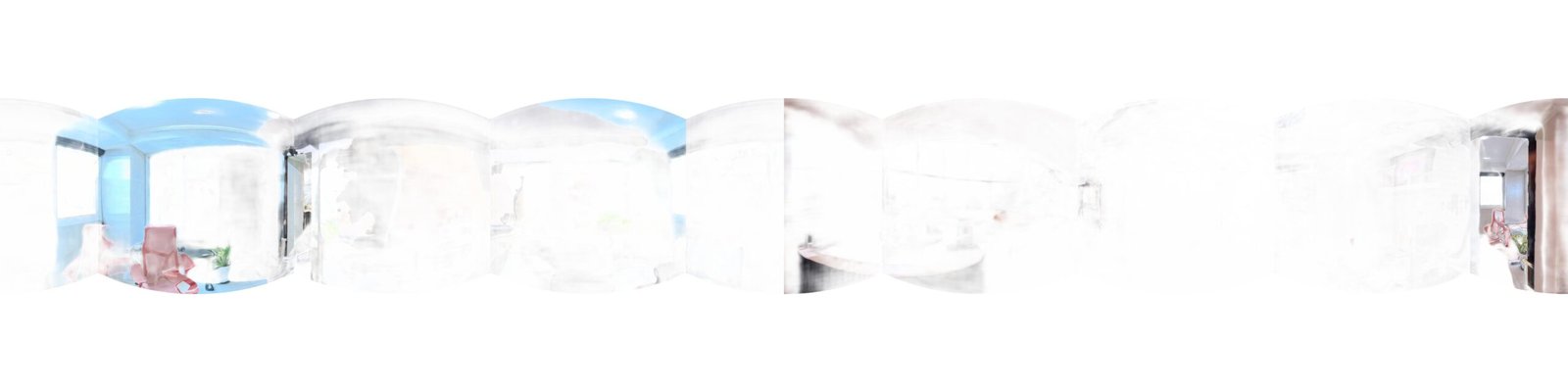
Glass, mirrors, and the sky are notorious problem-causers in computer vision. To an algorithm, a mirror on a wall often looks like a doorway into a completely identical room. A glass window might not register as a solid surface, but rather a hole leading to the outdoors. Furthermore, clouds in the sky move, meaning features captured on them cannot be used to calculate accurate angles between sequential photos.
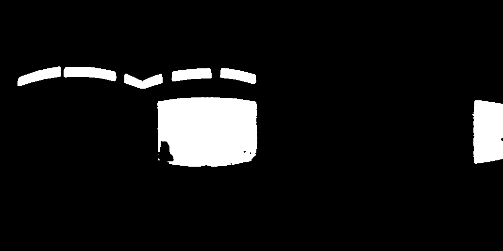
To prevent these elements from corrupting our data, we use an Open-Vocabulary Segmentation model, SAM 3.1, to identify and temporarily mask them out. Because SAM 3.1 natively understands equirectangular images, we can prompt it with natural language like “glass door, mirror, glass window, sky, clouds.” The model outputs precise black-and-white masks for these elements.
LightGlue and RoMa V2 use these masks to ignore those specific pixels prior to comparison. Without this step, two images on opposite sides of a solid wall might receive a strong match score simply because they share the same cloud formations in the sky. Removing these reflective and dynamic surfaces also drastically improves downstream 3D depth estimation, preventing the software from mistakenly calculating depth “through” a mirror or struggling with the refractive warping of a window.
Summary
This week began with a sluggish process that merely identified how a dataset could match together. It ended with a pipeline that is considerably faster, highly robust, and definitively identifies how everything should match together. By masking out common causes of false positives at the start, replacing CPU-intensive processes with optimized alternatives, and leveraging a GPU-based dense matcher for final validation, we eliminated the major bottlenecks. The resulting workflow now efficiently generates a minimum spanning tree where all connected paths represent their maximum confident pairs, ready for 3D reconstruction.